How to Monitor ML Models for Performance Decay and Data Shift | Complete Guide 2025
1. Introduction: The Quiet Killer of ML Models in Production
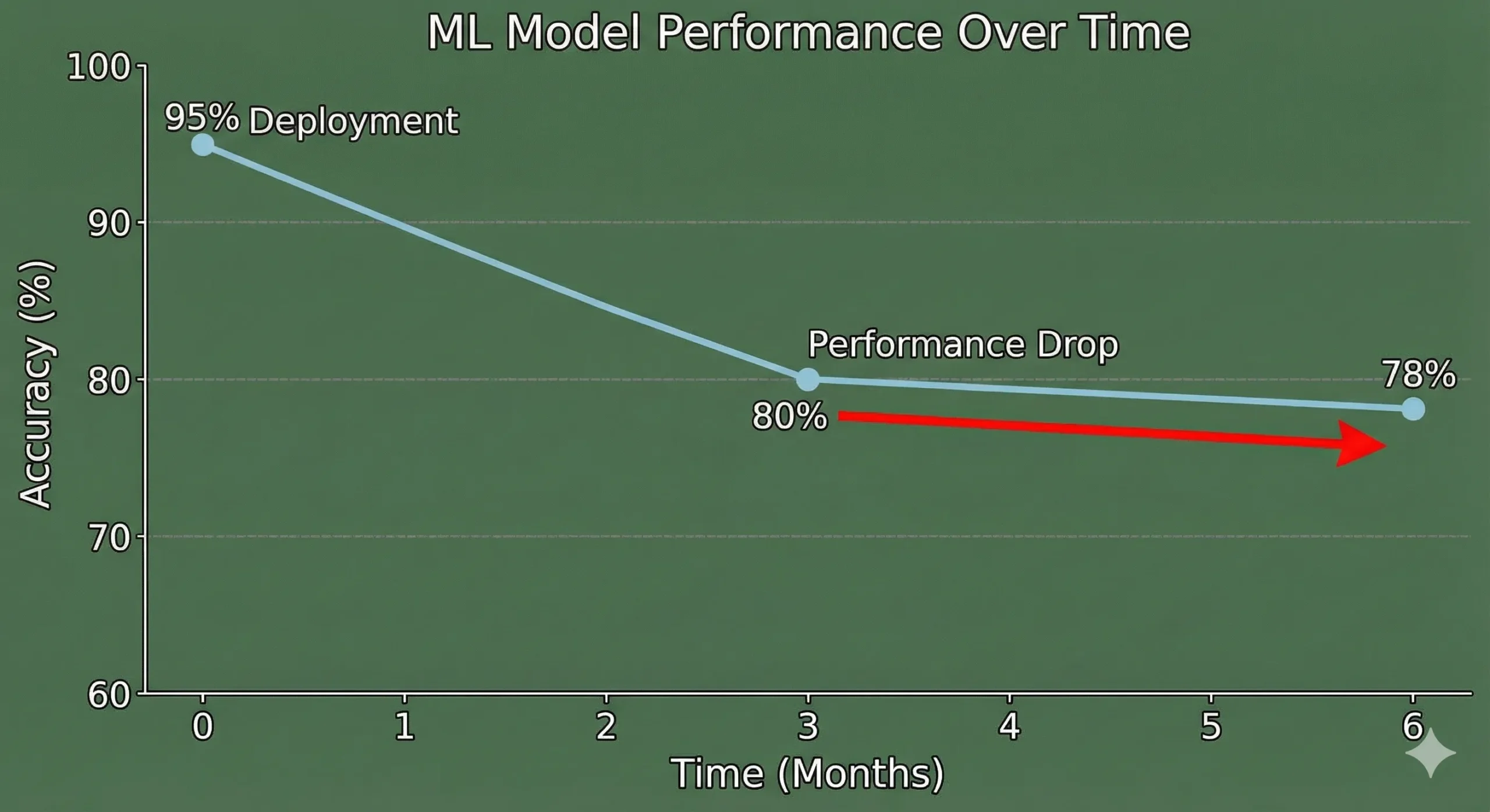
You build a machine learning model, test it thoroughly in your development environment, and then deploy it to production with confidence. The numbers look good. Your stakeholders are pleased. Three months later, your model’s accuracy drops by 15%, but no one notices until your business metrics start to fall.
This is what 91% of ML teams have to deal with. MIT and Harvard research shows that almost all production machine learning models get worse over time. But most teams don’t have a way to find this degradation until it’s too late and it’s already doing damage.
The uncomfortable truth is that your model isn’t the problem. Things changed in the world around it.
The ground is always shifting under your models’ feet, whether it’s because customers are acting differently, the market is changing, or the data pipeline is corrupting new features. You’re flying blind if you don’t have a good monitoring system in place. While you’re busy adding the next shiny feature, your model quietly breaks.
This guide tells you everything you need to know about keeping an eye on machine learning models that are in use. We’ll talk about data drift, concept drift, performance decay, how to find them, how to use Python, and the tools that really work. At the end, you’ll have a useful plan for keeping your models in good shape and protecting your business from hidden model failures.
Let’s get to work.
2. Understanding Model Decay: Why Models That Are Perfect Don’t Work
We need to know what’s really broken before we can talk about how to find problems.
Model decay is when a machine learning model’s performance gets worse over time, even though it worked perfectly when it was first put into use. Your model is fine. The information it sees has changed. It doesn’t work the same way in production as it did during training.
It’s like making a weather prediction model using data from the past ten years. That model works great for the next year. But by the third year, the weather patterns have changed a little. It’s not that your model is bad; it’s just that the climate it was trained on doesn’t exist anymore, so its predictions are less accurate.
The Actual Cost of Model Decay
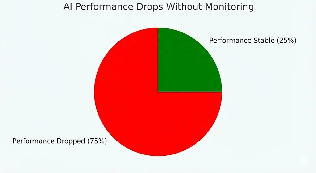
Not paying attention to model decay is more than just a technical issue. It has a direct effect on your business. Researchers at MIT looked at 32 datasets from a number of industries and found that:
75% of businesses saw AI performance drop when they didn’t keep an eye on it.
More than half said that AI mistakes cost them money.
Error rates on new data go up 35% when models are not changed for six months or more.
Some industries decay quickly (financial models break down in weeks), while others decay more slowly (image recognition stays stable for longer).
Decay is very important in systems that find fraud. If an insurance company’s fraud model is based on past fraud patterns, it might not catch newer, more advanced ways of committing fraud. Your company has already paid out fake claims by the time you realise that it’s not catching fraud well.
3. What’s Really Going On: Concept Drift vs. Data Drift
This is where most people get lost. They use the word “drift” in a lot of different ways. But there are actually different kinds of drift, and it’s important to know the difference because they need different fixes

Data Drift (Shift in Covariates)
When the input data distribution changes between training and production but the relationship between inputs and outputs stays the same, this is called data drift.
Picture that you made a model that can guess how much a house will cost. There were 80% suburban houses and 20% urban houses in your training data. Your real estate company starts to focus more on urban listings six months into production. Now, 60% of the data you enter is about urban properties.
Your model still knows how to guess prices. The model’s reasoning is still sound. But it’s getting a very different set of input data than it was trained on. That’s what data drift is.
For example, a credit scoring model that was trained on data from 2019 to 2020 suddenly has to deal with job patterns from 2024. The unemployment rate rose in different ways, the income distribution changed, and the way people borrowed money changed. The model sees inputs it has never seen before during training.
Concept Drift (Label Shift)
It’s harder to deal with concept drift because you can’t see it in your data. It happens when the link between the inputs and the target variable changes, even if the input data distribution looks the same.
A system for finding spam is a great example of this. Your model learnt how to tell the difference between spam and not spam by looking at how people spammed in 2022. But spammers got better. They are using new ways of writing, different sender addresses, and new ways of formatting. The input data may appear similar, but the definition of spam has fundamentally evolved.
A model for insurance fraud that was trained on common fraud patterns suddenly has to deal with new ways of committing fraud. Codes for medical care change. Rules in the state change. New kinds of claims come up. The model still gets medical claims that look the same, but the patterns that show fraud have changed completely.
| Drift Type | The Problem | The Fix |
| Data Drift | Input distribution changes. | Model might handle it, or might need retraining. |
| Concept Drift | The fundamental logic changes. | Must retrain with new data |
The catch is that concept drift almost always means that the model needs to be retrained. Data drift might not. Your model might be able to handle different input distributions without having to be retrained.
But what about concept drift? No amount of tuning your deployment will help if the relationship underneath it changes. You need to learn again with new data. That’s why it’s important to be able to tell the difference. It tells you what to do.
4. Two Ways to Find Model Decay
There are two main ways to tell if your model is getting worse: by looking at the ground truth and by looking at the input drift.
The Gold Standard: Ground Truth Monitoring
This is the easiest way to do it, but it needs data that is already labelled.
You keep an eye on your model’s performance metrics over time using real labels when they finally show up. If a customer buys something (the label arrives), you compare what the model said would happen with what actually happened.
How it works:
Model makes a guess, and the guess is saved with a timestamp.
The ground truth label comes (sometimes days or weeks later).
You figure out the accuracy, precision, recall, and F1-score of recent predictions.
Check the current metrics against the baseline, which is usually a 30-day rolling average.
If metrics drop below a certain level (usually 1–3% deterioration), send an alert.
Metrics to keep an eye on:
F1-score and accuracy for problems with classification
Mean Absolute Error (MAE) for regression
Precision and recall for the most important classes
AUC-ROC for problems with ranking
Custom business metrics like conversion rate, customer satisfaction, and so on
The problem is that labels often come late. It could take 30 to 60 days to find out if a transaction was really fraudulent. Ground truth could take months in a medical diagnosis system. Your model could be making terrible predictions while you wait.
Approach 2: Monitoring Input Drift (The Realistic Option)
You keep an eye on the input data itself when you can’t wait for ground truth. Performance is likely to get worse if the input data distribution changes a lot.
This compares the current input data distribution to the training data distribution using statistical tests. You’re looking for strange changes that show the model will have trouble soon.
How it works:
Find the statistical profile of the training data (baseline).
Keep calculating the statistical profile of the incoming production data.
Do a statistical test to see how the current situation compares to the baseline.
If divergence goes above the limit, send an alert.
Look into it or retrain ahead of time.
This works because of a basic idea: if your model sees data that is very different from what it was trained on, it will probably be less accurate.
5. Statistical Tests for Finding Data Drift
Now we get into the nitty-gritty details. Different statistical tests are better for different situations.
Kolmogorov-Smirnov (KS) Test
The KS test is one of the oldest and most reliable tests that doesn’t make any assumptions about the data to find changes in distributions.
What it does: It looks at two cumulative distribution functions and finds the greatest distance between them. Drift is found if this distance is statistically significant.
When to use: Great for features with numbers that don’t change. It’s quick and doesn’t make any assumptions about how the data is spread out.
The KS test is sensitive to changes in both location (mean) and shape. This makes it strong, but it can also give false positives in production environments where there is noise.
Python
from scipy.stats import ks_2samp

# Look at the training data and the current production data side by side.
statistic, p_value = ks_2samp(training_data['feature'], current_data['feature'])

# If p_value is less than 0.05, there is a significant drift.
if p_value < 0.05:
    print("Drift found!")
Population Stability Index (PSI)
PSI shows how much a population has changed compared to a baseline. For years, this has been the standard in credit risk.
The formula for PSI is:


Understanding:
PSI < 0.1: Very small change
PSI 0.1–0.25: Small change that should be watched
PSI > 0.25: Big change, look into it
PSI > 0.3: Big drift, probably need to retrain
When to use: Works well with both continuous and categorical features. Very helpful for keeping track of feature importance and credit risk.
The good thing about PSI is that it puts more weight on bins where the biggest changes in distribution happened, which makes sense to business people.
Python
import numpy as np

def calculate_psi(baseline, current, bins=10):
    # Put the data into bins
    baseline_counts = np.histogram(baseline, bins=bins)[0] + 0.0001 # to avoid dividing by zero
    current_counts = np.histogram(current, bins=bins)[0] + 0.0001

    # Change to percentages
    baseline_pct = baseline_counts / baseline_counts.sum()
    current_pct = current_counts / current_counts.sum()

    # Find PSI
    psi = np.sum((current_pct - baseline_pct) * np.log(current_pct / baseline_pct))
    return psi
Jensen-Shannon Divergence (JS)
JS divergence is a way to use math to find the distance between two probability distributions. It is symmetric (unlike KL divergence) and always finite, which makes it better for monitoring production.
When to use: Great for looking at different probability distributions. It works well with both continuous and discrete data. Not as sensitive to rare events as KS or PSI.
The good thing is that it is stronger than raw KL divergence. It captures differences in distribution smoothly, without the problems that KS has with sensitivity.
WhyLabs recommends the Hellinger Distance.
The Hellinger distance looks at the square root of probability distributions. This is what WhyLabs and other modern platforms suggest for keeping an eye on production.
Why it wins:
Symmetrical (doesn’t matter which way)
It works for both discrete and continuous features.
Stronger than JS divergence for data that is noisy in the real world
Not as likely to give false positives
The tradeoff is that it costs a little more to run than PSI, but the stability gains are worth it.
6. Case Study: Failure to Detect Insurance Fraud in the Real World
Let’s make this real. In January 2023, a mid-sized auto insurance company used a fraud detection model that was 92% accurate on their validation set. By March 2024, their fraud detection system was only catching 78% of fake claims.
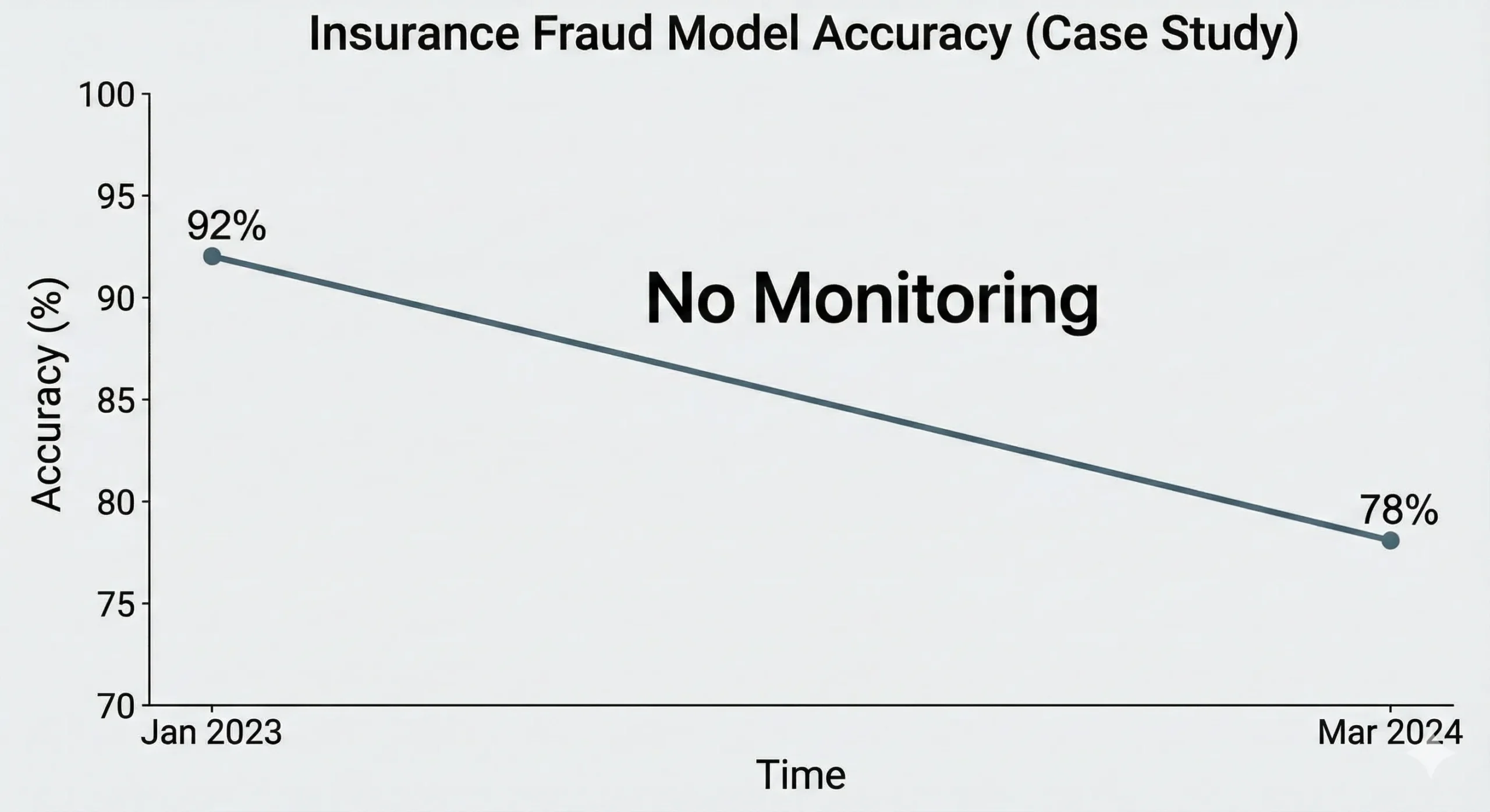
What happened? They didn’t put monitoring in place.
The Inquiry: When the CFO finally saw a rise in fake payout rates, they hired a consultant to look into it. This is what they found:
Data drift on numerical features: The average claim value went from $4,200 to $5,800. Not huge, but big enough to matter. The model learnt from old data that showed different patterns for bigger claims.
The medical codes had been changed: This caused concept drift in categorical features. There were new types of injuries added. In three places, state rules changed. The model’s learnt link between “injury code + claim amount → fraud” was no longer true.
Data pipeline corruption: A data engineer had changed the way the model calculated features six months before, but they hadn’t changed the model’s assumptions. There was a constant difference between the calculated claim ages.
The Price: The insurance company had already paid out about $2.3 million in fake claims that their model should have caught by the time they found it. They had to start over with their monitoring system and retrain people quickly.
What They Should Have Done:
Used PSI to keep an eye on feature distributions every day.
When PSI is greater than 0.2 on important features, set alerts.
Tracked model precision and recall every week, with a 30-day delay on the ground truth.
Watched how feature importance changed over time.
Set up automatic alerts for problems with data quality, like null rates and value ranges.
Set up a retraining trigger when accuracy fell 3% below the baseline.
This would have found the problem in weeks, not months.
7. The Full Stack for Building a Monitoring System
Okay, that’s enough theory. Let’s make something.
Step 1: Set Your Baseline
You need a baseline to compare against before you can find drift.
Python
from sklearn.datasets import load_breast_cancer
from sklearn.model_selection import train_test_split
import pandas as pd
import numpy as np

# Get your training data ready
X, y = load_breast_cancer(return_X_y=True)
X_train, X_test, y_train, y_test = train_test_split(
    X, y, test_size=0.2, random_state=42
)
X_train = pd.DataFrame(X_train)

# Make basic statistics
baseline = {
    "means": X_train.mean(),
    "stds": X_train.std(),
    "mins": X_train.min(),
    "maxs": X_train.max(),
    "quantiles": X_train.quantile([0.25, 0.5, 0.75])
}

print("Baseline set using training data")
Step 2: Set up basic drift detection
Keep an eye on your production data using the PSI method:
Python
def check_production_data(new_data, baseline_data, features, psi_threshold=0.2):
    """
    Check incoming production data for drift
    """
    drift_report = {}

    for feature in features:
        psi = calculate_psi(baseline_data[feature], new_data[feature], bins=10)

        drift_report[feature] = {
            "psi": psi,
            "drift_detected": psi > psi_threshold,
            'Action': 'investigate' if psi > psi_threshold else 'normal'
        }

    return drift_report

# Create fake production data with some drift
import numpy as np
production_data = pd.DataFrame(
    np.random.normal(loc=1.1, scale=1.2, size=(1000, X_test.shape[1])), # Distribution that has been shifted
    columns=X_train.columns
)

# Look for drift
report = check_production_data(production_data, X_train, X_train.columns)

# Show results
for feature, metrics in report.items():
    if metrics['drift_detected']:
        print(f"⚠️ Drift detected in {feature}: PSI = {metrics['psi']:.4f}")
    else:
        print(f"✓ {feature} stable: PSI = {metrics['psi']:.4f}")
Step 3: Keep an eye on performance metrics over time
Python
import json
from datetime import datetime, timedelta
from sklearn.metrics import f1_score, precision_score, recall_score, accuracy_score

class ModelMonitor:
    def __init__(self, model, performance_log_file='performance.json'):
        self.model = model
        self.log_file = performance_log_file
        self.history = []

    def log_predictions(self, X, y_true, y_pred=None):
        "Log predictions with real labels"
        if y_pred is None:
            y_pred = self.model.predict(X)

        metrics = {
            'timestamp': datetime.now().isoformat(),
            'accuracy': accuracy_score(y_true, y_pred),
            'precision': precision_score(y_true, y_pred),
            'recall': recall_score(y_true, y_pred),
            "f1": f1_score(y_true, y_pred),
            'sample_size': len(y_true)
        }

        self.history.append(metrics)

        # Store in a file
        with open(self.log_file, 'w') as f:
            json.dump(self.history, f)

        return metrics

    def check_performance_degradation(self, threshold=0.03, window_days=30):
        "Check to see if performance has gotten worse recently"
        if len(self.history) < 2:
            return {'degraded': False, 'reason': 'not enough data'}

        # Get metrics from the past
        recent_metrics = [
            m for m in self.history
            if datetime.fromisoformat(m['timestamp']) >
            datetime.now() - timedelta(days=window_days)
        ]

        if not recent_metrics:
            return {'degraded': False, 'reason': 'no_recent_data'}

        # Find the averages
        recent_avg = np.mean([m['accuracy'] for m in recent_metrics])

        # Get the older baseline
        older_metrics = [
            m for m in self.history
            if datetime.fromisoformat(m['timestamp']) <
            datetime.now() - timedelta(days=2 * window_days)
        ]

        if older_metrics:
            baseline_avg = np.mean([m['accuracy'] for m in older_metrics])
        else:
            baseline_avg = np.mean([m['accuracy'] for m in self.history[:5]])

        degradation = baseline_avg - recent_avg

        return {
            "degraded": degradation > threshold,
            "degradation_pct": degradation * 100,
            "recent_accuracy": recent_avg,
            'baseline_accuracy': baseline_avg,
            "action": "trigger_retrain" if degradation > threshold else "continue_monitoring"
        }

# How to use it
# monitor = ModelMonitor(model=your_model)
# sample_metrics = monitor.log_predictions(X_test, y_test)
# print(f"Latest metrics: {sample_metrics}")
Step 4: Set Up Alerts That Happen Automatically
Python
from datetime import datetime

class AlertSystem:
    def __init__(self):
        self.alerts = []

    def check_alerts(self, drift_report, performance_status):
        "Make alerts based on the results of monitoring"
        alerts = []

        # Drift warnings
        for feature, metrics in drift_report.items():
            if metrics['drift_detected']:
                alerts.append({
                    'level': 'warning',
                    "type": "data_drift",
                    'feature': feature,
                    'value': metrics['psi'],
                    'date': datetime.now().isoformat()
                })

        # Alert for performance problems
        if performance_status.get('degraded'):
            alerts.append({
                'level': 'critical',
                'type': 'performance_degradation',
                'degradation': performance_status['degradation_pct'],
                "action_needed": "retrain",
                'timestamp': datetime.now().isoformat()
            })

        self.alerts = alerts
        return alerts

    def send_notification(self, alerts):
        """Send alerts to your team via email, Slack, etc."""
        for alert in alerts:
            if alert['level'] == 'critical':
                print(f"🚨 CRITICAL: Found {alert['type']}!")
                # Send to email, Slack, or PagerDuty
                # slack_client.post_message(channel='#ml-alerts', text=alert)
            else:
                print(f"⚠️ WARNING: {alert['type']} in {alert.get('feature')}")

# How to Use
# alert_system = AlertSystem()
8. Using Evidently AI to Write Python Code
Modern teams use tools that were made for a specific purpose instead of making everything from scratch. Evidently AI is a great open-source Python library that does a lot of this work for you.
Setting Up and Installing
Bash
pip install evidently
Drift Report Made Easy
Python
from evidently.report import Report
from evidently.metric_preset import DataDriftPreset, TargetDriftPreset
from evidently.test_suite import TestSuite
from evidently.tests import TestDataDrift

import pandas as pd

# Get the data ready (reference = training, current = production)
reference_data = pd.DataFrame(X_train)
current_data = pd.DataFrame(X_test)

# Make a report on drift detection
drift_report = Report(metrics=[
    DataDriftPreset(),
    TargetDriftPreset()
])

drift_report.run(reference_data=reference_data, current_data=current_data)

# Store and show
drift_report.save_html("drift_report.html")

# Get metrics through code
drift_results = drift_report.as_dict()
# for metric in drift_results['metrics']:
#     print(metric['result'])
Dashboard for Real-Time Monitoring
Python
# from evidently.ui.workspace import Workspace
#
# # Set up a workspace for ongoing monitoring
# workspace = Workspace.create("my_ml_monitoring")
#
# # Set up a project for your model
# project = workspace.create_project("credit_fraud_model")
#
# # Add data for monitoring from time to time
# for week_num in range(10):
#     # Simulate data coming in every week
#     # weekly_data = make_weekly_data(week_num)
#
#     # Make a report
#     report = Report(metrics=[DataDriftPreset(), TargetDriftPreset()])
#     report.run(reference_data=reference_data, current_data=weekly_data)
#
#     # Log to workspace
#     project.add_report(report)
#
# # Go to http://localhost:8000 to see the dashboard.
9. Enterprise Tools: What Professionals Use
Dedicated tools make sense for teams that have more complicated needs or are working on a bigger project.
Comparison of the Best ML Model Monitoring Tools for 2025
| Tool | Best For | Pros | Cost |
| Evidently AI | Teams wanting open source freedom | Great for monitoring batches, easy Python integration, active community. | Free open-source; Cloud starts at $199/mo. |
| WhyLabs | Privacy-conscious companies | Uses whylogs to profile data without saving raw data (great for GDPR/HIPAA). Supports Hellinger distance. | Free tier (5 projects); Pro $299/mo. |
| Arize AI | Enterprise teams needing full visibility | Automatic root-cause analysis (finds why drift happened). Works with Databricks/Kubernetes. | Enterprise pricing. |
| Fiddler AI | Unstructured data (NLP/CV) | Unique vector monitoring for embeddings. Great explainability dashboard. | Business pricing. |
10. Use Case Monitoring Strategies
Not all monitoring is the same. What works for you will depend on your situation.
High-Latency Label Scenarios (Medical, Insurance)
You have to rely on input drift monitoring when ground truth labels come days or weeks later.
Plan: Using Hellinger distance or PSI to check feature distributions every day.
Threshold: Set the PSI threshold to 0.2 for a warning and 0.3 for a critical alert.
Routine: Weekly analysis of feature importance (do the same features still matter?).
Validation: Once the labels come in, monthly full accuracy checks are done.
When to retrain: PSI > 0.3 on 3+ key features, or actual accuracy drops by 3%+.
Real-Time Decision Scenarios (Fraud, Ad Tech)
When decisions are made right away and labels come quickly, it is possible to keep an eye on everything.
Plan: Tracking performance metrics in real time (updated every hour or day).
Segments: Tracking performance at the segment level (overall metrics can hide segment degradation).
Shadow Mode: Set up an A/B testing framework (the shadow model approach).
When to retrain: Primary accuracy metric drops > 2% from the 30-day baseline.
Batch Processing Scenarios (Analytics, Recommendations)
Big batch jobs that run every day or every week.
Plan: Reports on drift detection every week.
Stability: Checks for the stability of feature importance.
Trigger: Retrain when performance goes down for two to three weeks in a row.
11. How to Set Up Good Alert Thresholds
This is where theory meets practice. How do you know when to set off an alert?
The Alert System with Three Layers
Layer 1: Finding Drift
Warning: PSI 0.15
Critical Alert: PSI 0.3
Layer 2: Performance Loss
Warning: 2% drop from the 30-day average
Important: 5% drop from the baseline
Level 3: Quality of Data
Warning: The null rate goes up from 0.1% to 2%
Important: Any feature has more than 20% null values
Cutting Down on False Alarms: Static thresholds can make people tired of getting alerts. Modern monitoring platforms use dynamic thresholds:
Python
import numpy as np

def adaptive_threshold(historical_drift_values, percentile=90):
    """
    Set the threshold based on past drift values.
    A lot of businesses use the 90th percentile as "normal."
    """
    return np.percentile(historical_drift_values, percentile)
12. Automation and retraining triggers
Finding problems is only half the battle. You have to actually fix them.
When to Train Again
Retraining every so often: For stable domains, retraining every month on new data works well.
Retraining based on a trigger: Retrain when ground truth accuracy drops > X%, or data drift is found on important features.
Hybrid approach: Most experienced teams use periodic retraining (like every week) as a baseline and retraining based on triggers for emergencies.
Pipeline for automatic retraining:
Python
class AutomaticRetrainingPipeline:
    def __init__(self, monitor, model_trainer, version_control):
        self.monitor = monitor
        self.trainer = model_trainer
        self.version_control = version_control

    def should_retrain(self):
        """See if retraining needs to happen"""
        perf_status = self.monitor.check_performance_degradation(threshold=0.03)
        return perf_status.get('degraded', False)

    def retrain_and_validate(self, new_data):
        "Retrain the model and check it before deploying"
        # Learn from the most recent data
        new_model = self.trainer.train(new_data)

        # Check against the holdout test set
        validation_score = self.trainer.validate(new_model)

        # Compare to the current model of production
        production_model = self.version_control.get_current_version()
        production_score = production_model.score_on_validation_set()

        # Only deploy if the improvement is big (>1%)
        if validation_score > production_score * 1.01:
            # Optional: Deploy to the shadow model first
            # self.version_control.deploy_shadow(new_model, version=f"v{datetime.now().timestamp()}")
            return True, "Model ready for deployment"
        else:
            return False, f"Model didn't get better enough. New: {validation_score}, Current: {production_score}"
13. Dealing with Different Kinds of Drift
Not all drift needs the same reaction.
Drift that happens slowly vs. drift that happens suddenly
Gradual drift (Incremental): Happens over time. Customer preferences change week by week.
Answer: Regular monitoring catches it. Retraining every month or three months is usually enough.
Sudden drift: Happens overnight. A change in the rules, a market crash, or a viral event.
Response: Needs emergency monitoring and alerts every minute. Switch to a previous model or a conservative heuristic.
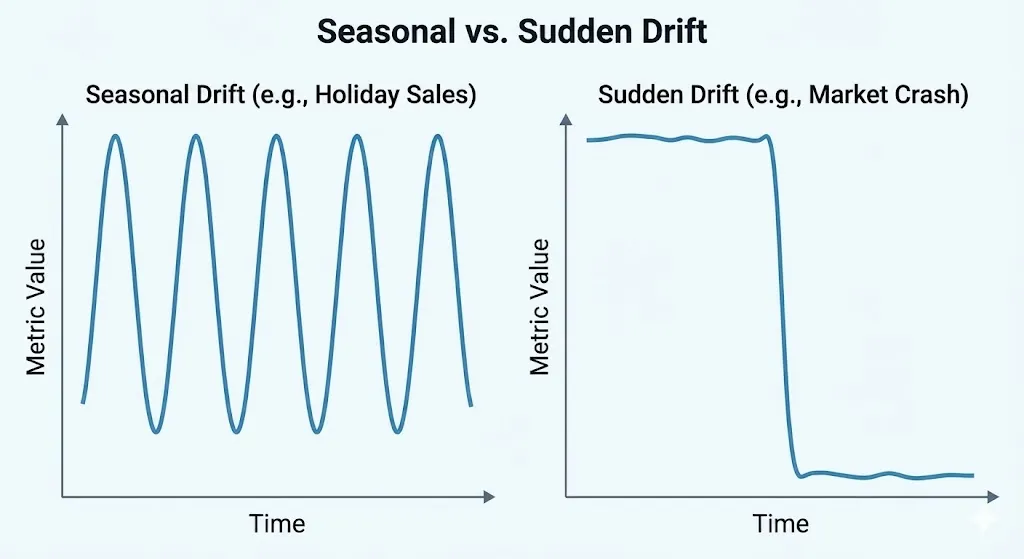
How to Deal with Seasonal Drift
You need to take this into account: some data has natural seasonality. For example, retail sales go up during the holidays, and fraud patterns change on weekends. Instead of a single baseline, use seasonal baselines.
Python
def make_seasonal_baseline(historical_data, date_column):
    """
    Set different baselines for each season.
    """
    baselines = {}

    # Sort by month or quarter
    # (Implementation logic to separate data by month)

    return baselines
14. Things to think about when monitoring in your industry
Different industries have different needs and drift characteristics.
Detecting Fraud in Financial Services: Rapid decay, concept drift is common, false negatives are expensive. Needs daily checks and real-time transaction monitoring.
AI in Healthcare and Medicine: Slow drift, extreme label latency. Needs long baselines (90+ days) and strict data quality checks.
E-Commerce and Suggestions: Seasonal patterns, user behavior changes. Optimize for business metrics (CTR) rather than pure model accuracy.
15. Questions that are asked a lot
Q1: How often should I check on my model? It depends on the stakes and the label latency. Daily monitoring is needed for high-stakes decisions like fraud or medical care. Batch recommendations can be made with weekly monitoring.
Q2: What does it mean when the PSI is 0.1 and 0.3? PSI is like a distance meter.
0.05–0.1: Very little drift.
0.1–0.25: Pay attention.
0.25–0.3: Big drift.
0.3+: A lot of drift, retrain right away.
Q3: Do I need to keep an eye on all the features or just the most important ones? Monitor the top 10 most important features, any features important for the business, and features that have caused problems in the past. This covers 80% of the risk.
Q4: How can I tell if it’s data drift or concept drift? Train a simple model on current data with a timestamp feature. If the timestamp is important, concept drift likely happened. If the timestamp isn’t important but distributions changed, it’s data drift.
Q5: Is it okay to use old labels for validation? Not really. Use recent labels for validation. If the labels are too late, use a holdout validation set from recent production data.
16. Creating a culture of monitoring
Half of the battle is having the right tools. The other half is having the right culture.
What teams that work well do:
Don’t just let the data science team keep an eye on things; everyone should be responsible for it.
Share the results with everyone via a dashboard.
When monitoring catches a problem early, celebrate the save, not the failure.
Run tests: Put fake drift into your monitoring system once a month to practise how to respond.
17. Conclusion: From Blind Deployment to Smart Monitoring
Your machine learning models aren’t things that you just deploy and forget about. They are living systems that work in a world that is always changing.
Without monitoring, that world changes around them. Quietly. Without being seen. Until your business metrics drop.
You catch these changes early if you keep an eye on them. You respond in a planned way, and you keep trusting your AI systems.
Here’s what you need to remember:
Start with the basics. Keep track of predictions and actual labels.
Add drift detection. Use Evidently or whylogs.
Automate the boring parts. Use Airflow or cloud schedulers.
Build up over time. From basic performance to automated retraining.
The teams that win with AI don’t have the best initial models; they have the best production model management.
18. Tools and resources to help you get started
Libraries that are open source:
Evidently AI: https://www.evidentlyai.com/
WhyLogs: https://whylogs.readthedocs.io/
Alibi Detect: Drift detection in particular
River: Learning online and finding drift
Cloud Platforms:
AWS SageMaker Model Monitor
Google Vertex AI Model Monitoring
Azure ML Model Monitoring
WhyLabs
Arize
Scientific Papers:
“Machine Learning Observability in Production” – IJCRT 2025
“Learning under Concept Drift: A Review” is a standard reference